This note continues the Chapter 0 reading on quotients and cell attachments. The main source is Allen Hatcher, Algebraic Topology, §1.1, “Basic Constructions,” printed pp. 25–27 (PDF pp. 34–36 in the author’s complete PDF). We stop at Example 1.4. Changing the basepoint and computing the fundamental group of a circle are separate reading tasks.
The question is: how can continuous paths in a space produce a group? We will first specify what may deform and what must stay fixed. Then we will pass from individual paths to their homotopy classes. Only after that step will concatenation satisfy the group laws as exact equalities.
There are three checkpoints: a path is a map; a path homotopy fixes its endpoints; an element of the fundamental group is a class of loops. This note expands Hatcher’s proofs, supplies explicit formulas for the changes of parameter, and checks their boundary conditions. The diagrams are original illustrations of those formulas.
0. Before starting: objects, notation, and continuity
Sets, points, and maps
A set is a collection of objects; an object in a set is an element. We write $x\in X$ to mean that $x$ is an element of a set $X$. The notation $A\subseteq X$ means that every element of a set $A$ belongs to $X$. The empty set, which has no elements, is written $\varnothing$. The union of two sets contains the elements in either set; their intersection contains the elements common to both. We denote intersection by $\cap$.
A map $f:A\to B$ assigns to each element $a$ of a set $A$ exactly one element $f(a)$ of a set $B$. Here $A$ is the domain and $B$ is the codomain. The arrow $\to$ records this direction; $f(a)$ is the value of the map at $a$. Two maps with the same domain and codomain are equal only if their values agree at every input.
The image of $f$ is the set of its values, written $f(A)=\{f(a):a\in A\}$. Braces $\{\ \}$ form a set; the colon inside the braces means “such that” or “as the variable ranges over.” Later, square brackets will have a different meaning.
Let $\mathbb R$ denote the real numbers. An interval $[a,b]$ contains the real numbers between $a$ and $b$, including both endpoints; $\leq$ means “less than or equal to.” For the moment, $a$ and $b$ are real numbers with $a\leq b$. Write
$$ I=[0,1]=\{s\in\mathbb R:0\leq s\leq1\}. $$Thus $I$ is the closed unit interval. The letter $s$ will measure position along a path. The letter $t$, also ranging over $I$, will measure progress through a deformation. An index such as the $0$ in $x_0$ is a label, not a power.
What topology contributes
A topological space is a set $X$ together with a collection of subsets called open sets. This collection contains $\varnothing$ and $X$, is closed under arbitrary unions, and is closed under finite intersections. A subset is closed if its complement is open. These conditions provide a precise language for continuity even when no distance formula is given. The usual topology on $\mathbb R$ consists of unions of open intervals, which exclude their endpoints.
For a map $f:A\to X$ and a subset $U\subseteq X$, its inverse image is
$$ f^{-1}(U)=\{a\in A:f(a)\in U\}. $$This notation does not assume that $f$ has an inverse map. A map between topological spaces is continuous if the inverse image of every open set is open. Equivalently, the inverse image of every closed set is closed. On Euclidean spaces this agrees with the usual definition from calculus.
If $A$ is a subset of a topological space $T$, its subspace topology consists of the intersections of $A$ with open sets of $T$. “Closed in $A$” is likewise relative to this topology; it need not mean closed in $T$. If $A$ is itself closed in $T$, however, every set closed in $A$ is closed in $T$. Indeed, such a set is the intersection of $A$ with a closed set of $T$.
We give $I$ its subspace topology from $\mathbb R$. For example, $[0,1/2)$ is open in $I$, although it is not open in $\mathbb R$. The product
$$ I\times I=\{(s,t):s\in I,\ t\in I\} $$is the unit square, with its usual topology as a subset of the plane. The first coordinate is $s$ and the second is $t$.
We will use two basic continuity facts. First, the composite of continuous maps is continuous: taking the inverse image under a composite amounts to taking two inverse images in succession, so openness is preserved at both steps. The notation $k\circ f$ means “apply $f$, then $k$,” whenever the values of $f$ lie in the domain of $k$. Second, the coordinate projections from the square to $I$, sending $(s,t)$ to $s$ or to $t$, are continuous. For example, the inverse image of an open subset $U$ of $I$ under the first projection is the strip $U\times I$, open in the square. We write $a\mapsto b$ to specify a rule that sends an input $a$ to an output $b$.
Term bridge · 连续映射. A picture of motion does not by itself establish continuity. Our task is to give a map on the whole interval or square and check that it is continuous there. In a two-parameter formula, joint continuity in $(s,t)$ is required.
The finite closed-set pasting lemma
We will use one elementary continuity result repeatedly. Let $T$ and $Y$ be topological spaces, and let $A,B$ be closed subsets of $T$ whose union is $T$. Suppose continuous maps $u:A\to Y$ and $v:B\to Y$ agree on their overlap $A\cap B$. They define a single continuous map $w:T\to Y$ by using $u$ on $A$ and $v$ on $B$.
Here is why. Let $C$ be a closed subset of $Y$. The inverse image $w^{-1}(C)$ is the union of $u^{-1}(C)$ and $v^{-1}(C)$. These are closed in $A$ and $B$, respectively, and hence closed in $T$ because $A$ and $B$ are closed in $T$. Their finite union is closed. The closed-set criterion therefore proves continuity of $w$. The same argument handles any finite number of closed pieces.
Reading rule. For every piecewise formula below, identify the closed pieces, check continuity on each piece, and verify that the formulas agree where pieces meet.
1. A path is a parametrized map
Let $X$ be a topological space. A path in $X$ is a continuous map
$$ f:I\longrightarrow X. $$Choose points $p,q\in X$. A path from $p$ to $q$ satisfies $f(0)=p$ and $f(1)=q$. We call these its initial and terminal points. They are allowed to coincide, and the path is allowed to pause, cross itself, or retrace part of its image. A map is injective if distinct inputs always have distinct outputs. Paths are not required to be injective.
The distinction between a map and its image matters. Let $\mathbb R^2$ denote the plane of ordered pairs of real numbers. Consider the paths $u,v:I\to\mathbb R^2$ given by
$$ u(s)=(s,0),\qquad v(s)=(s^2,0). $$They have the same image, namely the horizontal segment from $(0,0)$ to $(1,0)$, but they are different maps. For example,
$$ u(1/2)=(1/2,0),\qquad v(1/2)=(1/4,0). $$The difference is their schedule for visiting the segment. Thus “the same drawn curve” and “the same path” are different statements.
2. A homotopy of paths keeps two sides fixed
Let $f,g:I\to X$ be paths with the same initial point $p$ and terminal point $q$. A homotopy of paths relative to the endpoints is a continuous map
$$ H:I\times I\longrightarrow X $$satisfying four conditions:
$$ \begin{aligned} H(s,0)&=f(s),& H(s,1)&=g(s)&&\text{for every }s\in I,\\ H(0,t)&=p,& H(1,t)&=q&&\text{for every }t\in I. \end{aligned} $$The bottom edge of the parameter square records $f$; the top edge records $g$. The left edge stays at $p$; the right edge stays at $q$. The notation $H_t$ means the path at deformation time $t$, defined by $H_t(s)=H(s,t)$. The subscript $t$ is an index, not a derivative.
The symbol $\simeq$ means “is homotopic to”; “rel” abbreviates “relative to,” and $\{0,1\}$ is the pair of endpoints in the domain. When such a homotopy exists, we write
$$ f\simeq g\ \operatorname{rel}\{0,1\}. $$Throughout this note, homotopies between paths are relative to those endpoints, so we will often abbreviate the notation to $f\simeq g$.
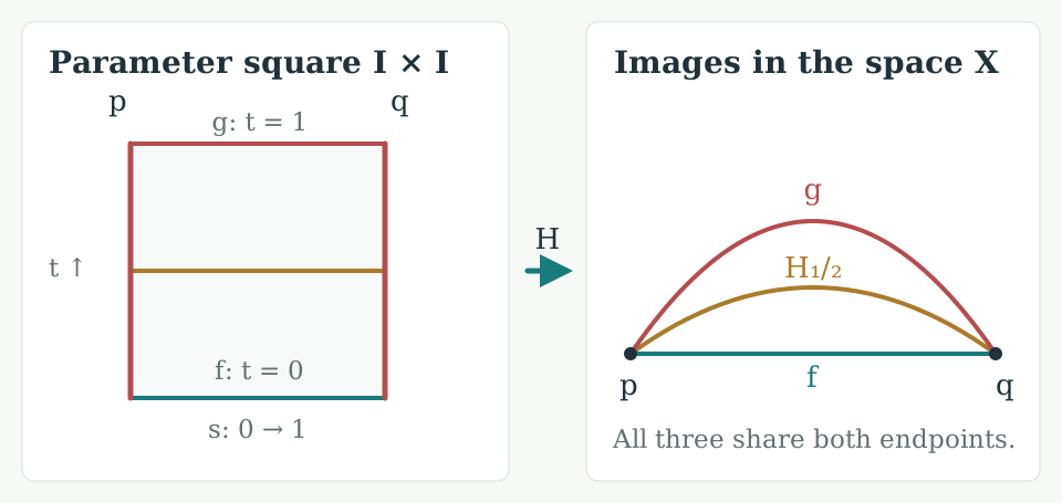
How to read it. The square on the left is the domain of $H$, not a region of $X$. A horizontal slice has constant $t$. Its image is one path in the right-hand picture. The three curves on the right have the same two endpoints; their colors identify three deformation times. Curves are drawn only in the image panel.
A first complete example: straight-line interpolation
Suppose now that $X=\mathbb R^2$. Addition and multiplication by a scalar are performed coordinate by coordinate. For instance, if $a=(a_1,a_2)$ and $b=(b_1,b_2)$ are points of the plane and $r$ is a real number, then $a+b=(a_1+b_1,a_2+b_2)$ and $ra=(ra_1,ra_2)$. These operations are continuous. Define
$$ H(s,t)=(1-t)f(s)+t g(s). $$We check every requirement:
- Values lie in the space. The displayed expression is a point of $\mathbb R^2$ for every $(s,t)\in I\times I$.
- Joint continuity. Composing the continuous maps $f,g$ with the projection $(s,t)\mapsto s$, then using continuous vector operations, gives a continuous map on the entire square.
- Initial path. At $t=0$, the formula gives $H(s,0)=f(s)$.
- Final path. At $t=1$, it gives $H(s,1)=g(s)$.
- Fixed initial point. Since $f(0)=g(0)=p$, we have $H(0,t)=(1-t)p+tp=p$.
- Fixed terminal point. Since $f(1)=g(1)=q$, we have $H(1,t)=q$ by the same calculation.
Thus any two paths in the plane with the same endpoints are homotopic relative to the endpoints. The first check is essential: the formula need not remain in a smaller space with a point removed.
Term bridge · 固定端点的同伦. Moving along a path means varying $s$ while $t$ is fixed. Deforming the path means varying $t$. These are different actions. For a homotopy of loops, the two vertical sides stay at the basepoint, but the bottom and top sides still trace the two loops; the entire boundary need not be constant.
3. Why homotopy classes are legitimate classes
Fix the space $X$ and endpoints $p,q$. A relation on a set is an equivalence relation when it has three properties: reflexivity, symmetry, and transitivity. Here $f,g,h$ are paths from $p$ to $q$. The symbol $\Longrightarrow$ means “implies.” In this case the three properties mean
$$ f\simeq f,\qquad f\simeq g\ \Longrightarrow\ g\simeq f,\qquad (f\simeq g\text{ and }g\simeq h)\ \Longrightarrow\ f\simeq h. $$We prove these properties rather than treating them as features of a drawing. This is Hatcher’s Proposition 1.2.
Reflexivity. Define $H(s,t)=f(s)$. It is continuous, begins and ends at $f$, and fixes the endpoints.
Symmetry. Suppose $H$ is a homotopy from $f$ to $g$. Define a new map $K$ by $K(s,t)=H(s,1-t)$. It is continuous because it is a composition of continuous maps. At $t=0$ it equals $g$, at $t=1$ it equals $f$, and its two vertical sides still take the values $p$ and $q$.
Transitivity. Suppose $H$ is a homotopy from $f$ to $g$ and $K$ is a homotopy from $g$ to $h$. Define
$$ L(s,t)= \begin{cases} H(s,2t),&0\leq t\leq1/2,\\ K(s,2t-1),&1/2\leq t\leq1. \end{cases} $$On the common edge $t=1/2$, both formulas equal $g(s)$. They are continuous on the two closed rectangles $I\times[0,1/2]$ and $I\times[1/2,1]$. The pasting lemma proves that $L$ is continuous on the square. Its bottom edge is $f$, its top edge is $h$, and both homotopies hold the same endpoints fixed. Hence $f\simeq h$.
We may therefore define the homotopy class of $f$ by
$$ [f]=\{g:I\to X:\ g\text{ is a path from }p\text{ to }q\text{ and }g\simeq f\}. $$The square brackets $[f]$ mean a set of equivalent paths, not the image $f(I)$ and not a selected “best” path. Any particular path in this class is a representative of the class. The symbol $\Longleftrightarrow$ means that each statement implies the other. By the equivalence-relation properties,
$$ [f]=[g]\quad\Longleftrightarrow\quad f\simeq g. $$In one direction, homotopic paths have exactly the same equivalent paths. In the other, $f\in[f]=[g]$ implies $f\simeq g$.
4. Following one path and then another
Choose a third point $r\in X$. Let $f$ be a path from $p$ to $q$, and let $g$ be a path from $q$ to $r$. Their concatenation, denoted $f*g$, is the path
$$ (f*g)(s)= \begin{cases} f(2s),&0\leq s\leq1/2,\\ g(2s-1),&1/2\leq s\leq1. \end{cases} $$The symbol $*$ means “first follow the path on the left, then the path on the right.” Hatcher writes this product as $fg$; we insert $*$ to distinguish it from ordinary numerical multiplication. During the first half of the interval, $2s$ ranges from $0$ to $1$. During the second half, $2s-1$ does the same for $g$.
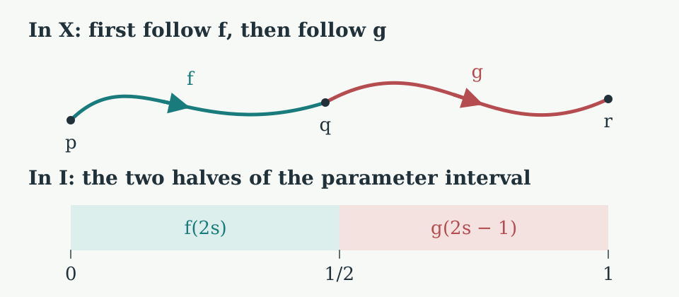
How to read it. The upper drawing represents points of $X$. The lower bar is the parameter interval, not a segment of $X$. Both halves have length $1/2$; this says nothing about the geometric lengths of $f$ and $g$.
The centered dot $\cdot$ in the numerical calculation below denotes multiplication of real numbers. Three checks establish that this formula defines a path. Each argument lies in $I$ on its assigned half. Both pieces are continuous. At $s=1/2$ they agree because
$$ f(2\cdot1/2)=f(1)=q=g(0)=g(2\cdot1/2-1). $$The pasting lemma applies to the closed intervals $[0,1/2]$ and $[1/2,1]$. The endpoints of the resulting path are
$$ (f*g)(0)=p,\qquad(f*g)(1)=r. $$The matching-endpoint condition is part of the construction. A pair of arbitrary paths cannot necessarily be concatenated this way.
For later use, define two further paths. The constant path at $p$ is the map $c_p:I\to X$ with $c_p(s)=p$ for every $s$. The reverse path of $f$ is the map $\overline f:I\to X$ given by $\overline f(s)=f(1-s)$. The bar denotes reversal of the parameter; it does not mean an inverse function. The reverse path goes from $q$ to $p$, and reversing it twice returns exactly $f$.
5. Why the product does not depend on representatives
An operation on classes is not valid until changing representatives gives the same answer. This is what well defined means here.
Let $f_0,f_1$ be paths from $p$ to $q$, and let $g_0,g_1$ be paths from $q$ to $r$. The subscripts label paths. Suppose $H$ is an endpoint-fixed homotopy from $f_0$ to $f_1$, and $K$ is one from $g_0$ to $g_1$. Define
$$ P(s,t)= \begin{cases} H(2s,t),&0\leq s\leq1/2,\\ K(2s-1,t),&1/2\leq s\leq1. \end{cases} $$At the seam $s=1/2$, both values equal $q$, since $H(1,t)=q=K(0,t)$ for every $t$. The two formulas are continuous on the closed rectangles $[0,1/2]\times I$ and $[1/2,1]\times I$, so they paste continuously. The remaining conditions are
$$ \begin{aligned} P(s,0)&=(f_0*g_0)(s),&P(s,1)&=(f_1*g_1)(s),\\ P(0,t)&=p,&P(1,t)&=r. \end{aligned} $$Thus $f_0*g_0\simeq f_1*g_1$. In the language of classes,
$$ [f_0]=[f_1],\ [g_0]=[g_1] \quad\Longrightarrow\quad [f_0*g_0]=[f_1*g_1]. $$This proof is different from transitivity in §3. There we joined two deformations in $t$; here we join two paths in $s$ at every deformation time. The two coordinate directions have different jobs.
6. Loops, a basepoint, and the group we want
Choose a point $x_0\in X$. A space with a chosen point is called a based space, written $(X,x_0)$, and $x_0$ is its basepoint. A loop based at $x_0$ is a path $f:I\to X$ for which
$$ f(0)=f(1)=x_0. $$In particular, $c_{x_0}$ is a loop. Every two loops at $x_0$ can be concatenated, and their product is again a loop at $x_0$.
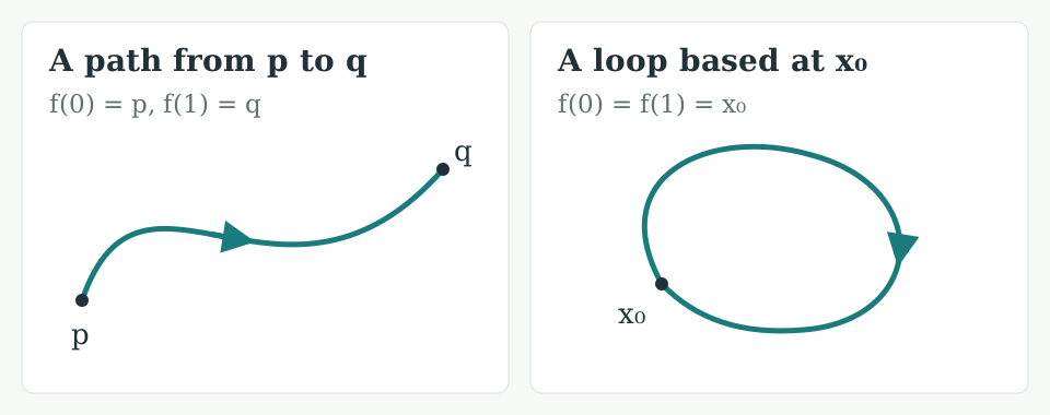
How to read it. The arrow indicates increasing path parameter. In the right panel the curve actually closes at $x_0$. Having the same start and end does not require visiting any other point only once.
We will write $\pi_1(X,x_0)$ for the set of endpoint-fixed homotopy classes of loops at $x_0$. The notation $\pi_1$ is read “pi one”; it is a name, not multiplication by the circle constant. Explicitly, define
$$ \pi_1(X,x_0)=\{[f]:f\text{ is a loop in }X\text{ based at }x_0\}. $$This set will become the fundamental group, also called the first homotopy group. At this point we have a set and a candidate multiplication. We will prove that they form a group.
A binary operation on a set assigns one element of that set to each ordered pair of its elements. A group is a set with a binary operation that is associative, has a two-sided identity, and gives each element a two-sided inverse. Concretely, for elements $a,b,d$, associativity means $(ab)d=a(bd)$; an identity $e$ satisfies $ea=ae=a$; an inverse $b$ for $a$ satisfies $ab=ba=e$. Juxtaposition in these three formulas denotes the proposed group operation, not numerical multiplication.
For loop classes, we now use the dot $\cdot$ to denote a new operation. On our set of loop classes we define
$$ [f]\cdot[g]=[f*g]. $$The preceding section proves that it is well defined; the common basepoint ensures it is defined for every pair. We still owe proofs of associativity, identity, and inverses.
7. A change of parameter preserves a path class
Let $f:I\to X$ be a path from $p$ to $q$. Let $\varphi:I\to I$ be a continuous map satisfying $\varphi(0)=0$ and $\varphi(1)=1$. The Greek letter $\varphi$, read “phi,” names a map of the parameter interval. Recall that $\circ$ denotes composition, so
$$ (f\circ\varphi)(s)=f(\varphi(s)). $$This is another path from $p$ to $q$. We will prove $f\circ\varphi\simeq f$.
Define, for each $t\in I$, a parameter map $\varphi_t:I\to I$ by
$$ \varphi_t(s)=(1-t)\varphi(s)+ts. $$The two numbers $\varphi(s)$ and $s$ lie in $I$. Their weighted average lies in $I$ because
$$ 0\leq(1-t)\varphi(s)+ts\leq(1-t)+t=1. $$Consequently the following formula is defined everywhere on the square:
$$ R(s,t)=f\bigl((1-t)\varphi(s)+ts\bigr). $$The expression inside $f$ is jointly continuous, so $R$ is continuous by composition. Its bottom and top edges are $f\circ\varphi$ and $f$, respectively. Since $\varphi(0)=0$ and $\varphi(1)=1$, its vertical edges are fixed at $p$ and $q$. This proves the claim.
Where the linear interpolation takes place. We interpolated between two real parameters inside $I$, then applied $f$. We did not add points of $X$. This is why the proof works for every topological space $X$. The maps used below are nondecreasing and describe pauses or changes of schedule. The lemma itself does not require $\varphi$ to be injective or nondecreasing.
8. The constant loop gives a two-sided identity
For a path $f$ from $p$ to $q$, the product $f*c_q$ follows $f$ during the first half of the interval, then stays at $q$. Define the continuous parameter map
$$ \varphi_R(s)= \begin{cases} 2s,&0\leq s\leq1/2,\\ 1,&1/2\leq s\leq1. \end{cases} $$The subscript $R$ labels a constant path placed on the right. The pieces agree at $s=1/2$, and the endpoint values are $0$ and $1$. The concatenation formula gives the exact equality
$$ f*c_q=f\circ\varphi_R. $$Applying §7 gives $f*c_q\simeq f$. Likewise, define
$$ \varphi_L(s)= \begin{cases} 0,&0\leq s\leq1/2,\\ 2s-1,&1/2\leq s\leq1. \end{cases} $$The subscript $L$ labels a constant path placed on the left. The map is continuous, fixes the interval endpoints, and satisfies $c_p*f=f\circ\varphi_L$. Thus $c_p*f\simeq f$ as well.
For a loop based at $x_0$, both $p$ and $q$ equal $x_0$. Set $e=[c_{x_0}]$. The two path homotopies yield the exact class identities
$$ [f]\cdot e=[f],\qquad e\cdot[f]=[f]. $$Therefore $e$ is a two-sided identity. The constant loop usually changes a representative’s time schedule when concatenated; it leaves its class unchanged.
9. Associativity: write down the two schedules
Let $f,g,h$ be loops at $x_0$. Define two loop maps
$$ a=(f*g)*h,\qquad b=f*(g*h). $$Expanding the concatenation definition gives
$$ a(s)= \begin{cases} f(4s),&0\leq s\leq1/4,\\ g(4s-1),&1/4\leq s\leq1/2,\\ h(2s-1),&1/2\leq s\leq1, \end{cases} $$and
$$ b(s)= \begin{cases} f(2s),&0\leq s\leq1/2,\\ g(4s-2),&1/2\leq s\leq3/4,\\ h(4s-3),&3/4\leq s\leq1. \end{cases} $$They follow the same paths in the same order, but allocate different fractions of the interval. In general they are not equal as maps.
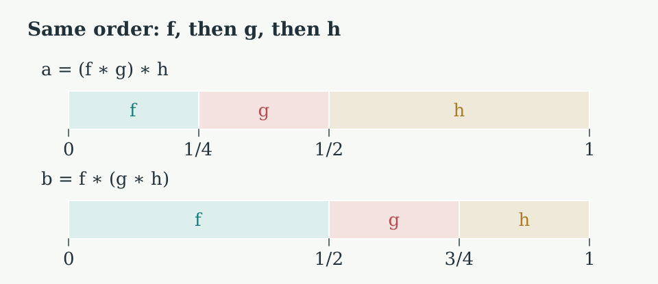
How to read it. Both bars represent the same interval $I$. The widths show time allocations, not distances. To obtain $b$ by evaluating $a$ on a new schedule, send the breakpoints $0,1/2,3/4,1$ of $b$ to the breakpoints $0,1/4,1/2,1$ of $a$.
Here is that schedule explicitly. Define
$$ \varphi(s)= \begin{cases} s/2,&0\leq s\leq1/2,\\ s-1/4,&1/2\leq s\leq3/4,\\ 2s-1,&3/4\leq s\leq1. \end{cases} $$It takes the values $0,1/4,1/2,1$ at those four breakpoints. The pieces agree at their joins, so the pasting lemma makes $\varphi$ continuous. It maps $I$ into $I$ and fixes both endpoints.
Check the identity $a\circ\varphi=b$ on each piece. For $0\leq s\leq1/2$, we have $a(\varphi(s))=f(4(s/2))=f(2s)$. For $1/2\leq s\leq3/4$, it is $g(4(s-1/4)-1)=g(4s-2)$. For $3/4\leq s\leq1$, it is $h(2(2s-1)-1)=h(4s-3)$. These are exactly the three pieces of $b$.
The lemma in §7 therefore supplies the continuous, endpoint-fixed homotopy
$$ A(s,t)=a\bigl((1-t)\varphi(s)+ts\bigr) $$from $b$ to $a$. By symmetry, $a\simeq b$ also. Passing to classes gives
$$ ([f]\cdot[g])\cdot[h] =[(f*g)*h] =[f*(g*h)] =[f]\cdot([g]\cdot[h]). $$This is associativity as an equality in the set of classes. It is not strict associativity of the binary concatenation formula on individual paths.
10. Reversing a loop gives its inverse
Let $f$ again be a path from $p$ to $q$. The product $f*\overline f$ goes out along $f$ and returns along exactly the same route. We will contract it to $c_p$ without assuming any geometry or vector operations in $X$.
Define a continuous real-valued map $v:I\to I$ by
$$ v(s)= \begin{cases} 2s,&0\leq s\leq1/2,\\ 2-2s,&1/2\leq s\leq1. \end{cases} $$The pieces agree at $1/2$. Its values increase from $0$ to $1$, then decrease to $0$. Thus $f\circ v=f*\overline f$ exactly. Now define
$$ Q(s,t)=f\bigl((1-t)v(s)\bigr). $$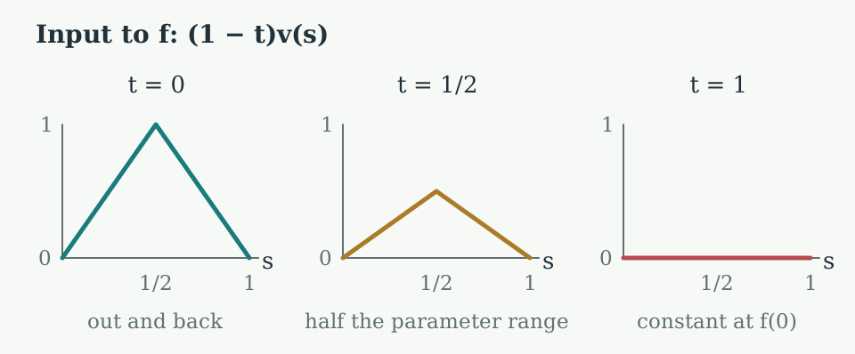
How to read it. Each panel graphs a real parameter supplied to $f$; it does not draw $X$. The horizontal coordinate is $s$. The vertical coordinate is $(1-t)v(s)$. As $t$ increases, the maximum parameter reached decreases to zero. Applying $f$ turns this into a shorter outward journey followed by the same journey in reverse.
We verify the homotopy:
- Since $0\leq v(s)\leq1$ and $0\leq1-t\leq1$, the argument of $f$ lies in $I$.
- The map $(s,t)\mapsto(1-t)v(s)$ is continuous, and so is its composition with $f$.
- At $t=0$, we have $Q(s,0)=f(v(s))=(f*\overline f)(s)$.
- At $t=1$, we have $Q(s,1)=f(0)=p$, so the final path is $c_p$.
- Since $v(0)=v(1)=0$, both endpoints stay at $p$ throughout.
This proves $f*\overline f\simeq c_p$. Apply exactly the same construction to the path $\overline f$, whose initial point is $q$. Reversing $\overline f$ gives $f$, so we also obtain $\overline f*f\simeq c_q$.
For loops at $x_0$, define the proposed inverse of the class $[f]$ to be $[\overline f]$. This is independent of the representative: if $H$ is a homotopy from $f$ to $g$, then $(s,t)\mapsto H(1-s,t)$ is an endpoint-fixed homotopy from $\overline f$ to $\overline g$. Both class products therefore satisfy
$$ [f]\cdot[\overline f]=e, \qquad [\overline f]\cdot[f]=e. $$This verifies both inverse identities. The customary notation $[f]^{-1}$ means this group inverse, not an inverse function of the path.
11. The construction is now a group
We have completed Hatcher’s Proposition 1.3. The fundamental group of $X$ at $x_0$ is the set $\pi_1(X,x_0)$ with multiplication $[f]\cdot[g]=[f*g]$.
| Requirement | What had to be checked | Where it was proved |
|---|---|---|
| Classes exist | Endpoint-fixed homotopy is an equivalence relation | §3 |
| Multiplication is well defined | Homotopic representatives give homotopic products | §5 |
| Every pair can be multiplied | All loops have the same basepoint | §6 |
| Two-sided identity | The constant loop changes only the class representative | §8 |
| Associativity | The two schedules are homotopic | §9 |
| Two-sided inverses | An excursion followed by its reverse contracts | §10 |
The distinction to retain. The individual paths may have different schedules and fail to be equal. Their homotopy classes are equal when an allowed homotopy connects the paths. Consequently the group laws hold as exact equalities of classes.
We have constructed a group; we have not yet proved the general theorems describing how it behaves under maps or homotopy equivalences of spaces. Those require further arguments in the subsequent reading.
12. A complete calculation: convex spaces
Let $n$ be a positive integer, and let $\mathbb R^n$ denote the space of ordered $n$-tuples of real numbers with its usual Euclidean topology. Vector operations are coordinatewise, just as in the plane. A subset $C\subseteq\mathbb R^n$ is convex if, for every $u,v\in C$ and every $t\in I$, the point $(1-t)u+tv$ lies in $C$. In words, the entire straight segment between any two points of $C$ remains in $C$.
Choose $x_0\in C$, and let $f:I\to C$ be any loop at $x_0$. Define
$$ H(s,t)=(1-t)f(s)+t x_0. $$Convexity ensures that the values remain in $C$. The vector operations make $H$ continuous as a map into $\mathbb R^n$, hence continuous into the subspace $C$ because all its values lie in $C$. Its bottom edge is $f$ and its top edge is $c_{x_0}$. At $s=0$ and $s=1$, the value is $(1-t)x_0+t x_0=x_0$. Thus every loop belongs to the same class as the constant loop.
It follows that
$$ \pi_1(C,x_0)=\{[c_{x_0}]\}. $$A group with one element is called the trivial group. Hatcher writes it as $0$; we have displayed its sole element to keep the meaning explicit. The whole space $\mathbb R^n$ is convex, so this includes the calculation for $\mathbb R^n$.
Why removing one point changes the argument
The symbol $\setminus$ means set difference: remove from the first set all the elements of the second. Let $o=(0,0)$ be the origin and let $Y=\mathbb R^2\setminus\{o\}$ be the plane with that point removed. Define paths $u,v:I\to Y$ by
$$ u(s)=(2s-1,\ 4s(1-s)),\qquad v(s)=(2s-1,\ -4s(1-s)). $$Both go from $(-1,0)$ to $(1,0)$ and avoid the origin: the first coordinate vanishes only at $s=1/2$, where the second coordinate is $1$ or $-1$. However, the proposed interpolation $H(s,t)=(1-t)u(s)+t v(s)$ has
$$ H(1/2,1/2)=(0,0), $$which is outside $Y$. It therefore does not define a homotopy in $Y$.
This proves only that this particular formula fails. It does not prove that no other homotopy exists. Proving nonexistence of homotopies is a different task; it is part of what makes the circle calculation on the following pages substantial.
13. Exercises, with checks
The exercises test definitions and the formulas already proved. Attempt each one before expanding its check.
Exercise 1. Same image, different maps
For the paths $u(s)=(s,0)$ and $v(s)=(s^2,0)$ in §1, write an endpoint-fixed homotopy from $u$ to $v$.
Check the formula and all four edges
Use $H(s,t)=((1-t)s+ts^2,0)$. It is polynomial in the two coordinates, hence continuous. The bottom and top edges give $u$ and $v$. At $s=0$ its value is $(0,0)$; at $s=1$ its value is $(1,0)$, independently of $t$.
Exercise 2. Reversal is not inversion of a function
For a path $f$ from $p$ to $q$, calculate the endpoints of $\overline f$ and show that $\overline{\overline f}=f$.
Check the endpoint values and the composition
They are $\overline f(0)=f(1)=q$ and $\overline f(1)=f(0)=p$. For every $s$, reversing twice gives $f(1-(1-s))=f(s)$. No injectivity assumption is needed.
Exercise 3. Check associativity at a specific time
Use the loops $a,b$ and parameter map $\varphi$ defined in §9. At $s=5/8$, which original path is being followed by $b$? Verify $a(\varphi(5/8))=b(5/8)$.
Check the two schedules
Since $1/2\leq5/8\leq3/4$, the formula for $b$ gives $g(4(5/8)-2)=g(1/2)$. Also $\varphi(5/8)=5/8-1/4=3/8$. This lies in the second interval for $a$, and $a(3/8)=g(4(3/8)-1)=g(1/2)$.
Exercise 4. Check the inverse homotopy halfway through
For the map $Q$ in §10, compute $Q(0,1/2)$, $Q(1/2,1/2)$, and $Q(1,1/2)$.
Check how much of the original path remains
The values are $f(0)=p$, $f(1/2)$, and $f(0)=p$. At deformation time $1/2$, the excursion travels only to parameter $1/2$ of $f$ before returning. This is a statement about parameters, not half of a geometric distance.
Exercise 5. Why do we need classes?
Explain why $f*c_q$ need not equal $f$ as maps, even though $[f*c_q]=[f]$.
Check a concrete representative
In the real line, take $f(s)=s$, so $q=1$. At $s=1/4$, $(f*c_q)(1/4)=f(1/2)=1/2$, whereas $f(1/4)=1/4$. The maps are different. The homotopy in §8 proves equality of their classes.
Exercise 6. A failing formula is not a nonexistence proof
For the space $Y$ and paths $u,v$ in §12, identify precisely which requirement the straight-line formula violates. Explain why that does not settle whether $u$ and $v$ are homotopic in $Y$.
Check the quantifier
The formula has a value outside its stated codomain $Y$, so it is not a map $I\times I\to Y$. Rejecting one proposed formula says nothing by itself about all possible maps with the required boundary conditions.
Source and the next reading
The primary source is Allen Hatcher, Algebraic Topology, author’s download page. In §1.1, printed p. 25 introduces paths and linear homotopies; p. 26 proves that path homotopy is an equivalence relation and defines loop classes; p. 27 proves the group axioms and gives the convex-space example. These correspond to Example 1.1, Propositions 1.2–1.3, and Example 1.4. The explicit formulas here expand the arguments; the inverse homotopy uses a shrinking parameter excursion rather than copying Hatcher’s diagram word for word.
The next reading is printed p. 28: path components, change of basepoint, group homomorphisms and isomorphisms, and simple connectivity. Each algebraic term will be defined before it is used. Only after those ideas are established will we turn to the fundamental group of the circle on p. 29.