This note continues the reading of Allen Hatcher, Algebraic Topology, Chapter 0, pp. 5–13 (PDF pp. 14–22). The first note treated homotopies and deformation retractions. Here the basic question changes: how can a space be built by taking simple pieces and specifying exactly how their boundaries are identified? The answer is the quotient construction, followed by the inductive language of CW complexes.
The order matters. An attaching map is not a picture of a disk glued to a space; it is a continuous map whose quotient defines the glued space.
1. Quotient spaces
Let $X$ be a topological space and let $\sim$ be an equivalence relation on its underlying set. The quotient set $X/{\sim}$ consists of the equivalence classes $[x]$. The quotient map is
$$ q:X\longrightarrow X/{\sim},\qquad q(x)=[x]. $$The quotient topology is defined by the rule
$$ U\subseteq X/{\sim}\text{ is open} \quad\Longleftrightarrow\quad q^{-1}(U)\subseteq X\text{ is open}. $$Thus a set downstairs is open precisely when its full collection of representatives upstairs is open. A map $F:X/{\sim}\to Y$ is continuous exactly when $F\circ q:X\to Y$ is continuous. This is the universal property that makes quotient spaces useful: continuity after the identification can be checked before the identification.
Term bridge. An equivalence relation is a rule that is reflexive, symmetric, and transitive; it decides which points become one point. A quotient space is the resulting set of classes with the quotient topology. The word universal refers to the factorization test above: a map out of the quotient is continuous exactly when its composite with $q$ is continuous.
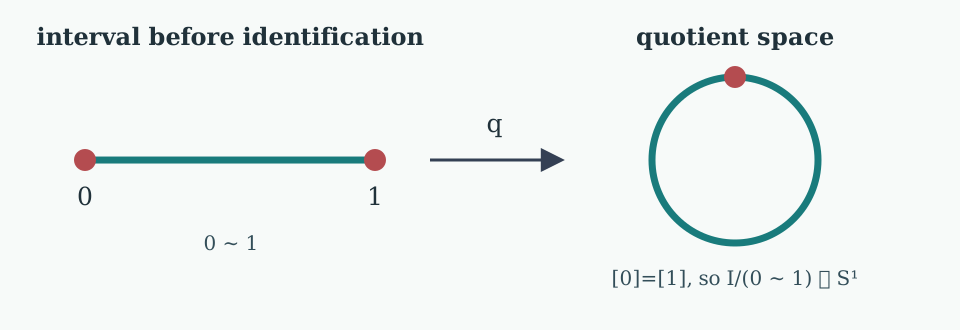
How to read it. The left side records the equivalence relation; the right side is not drawn by bending the interval, but obtained by identifying the two red endpoints.
The circle from an interval. On $I=[0,1]$, identify $0\sim1$ and leave all other points distinct. The map $q:I\to S^1$ given by $q(t)=e^{2\pi i t}$ is constant on equivalence classes, so it factors through a continuous map $\bar q:I/{\sim}\to S^1$. It is bijective: two parameters give the same point of $S^1$ exactly when they differ by an integer. Since $I/{\sim}$ is compact and $S^1$ is Hausdorff, $\bar q$ is a homeomorphism. The endpoint identification is the construction; the circle is its resulting space.
The same quotient construction gives
$$ D^n/\partial D^n\cong S^n. $$Here $D^n=\{x\in\mathbb R^n:\lVert x\rVert\leq1\}$ is the closed unit disk and $\partial D^n=S^{n-1}$ is its boundary. Collapse the entire boundary to one point. For $x\neq0$, put
$$ F(x)=\left(\sin(\pi\lVert x\rVert)\frac{x}{\lVert x\rVert},-\cos(\pi\lVert x\rVert)\right)\in S^n, $$and set $F(0)=(0,\ldots,0,-1)$. The boundary is sent to $(0,\ldots,0,1)$, so $F$ factors through the quotient. The induced map is a continuous bijection from the compact space $D^n/\partial D^n$ to the Hausdorff space $S^n$, hence a homeomorphism. The formula makes the identification explicit; the quotient property supplies continuity.
The notation $X/A$ means the quotient obtained by identifying every point of a subspace $A\subseteq X$ to one point while leaving points of $X\setminus A$ distinct. This operation is sensitive to the subspace topology: the map $X\to X/A$ is continuous by definition, but the quotient need not resemble a subspace of $X$.
2. Attaching one cell
Let $X$ be a space, let $A\subseteq Y$ be a subspace, and let $f:A\to X$ be continuous. The space obtained by attaching $Y$ to $X$ along $f$ is
$$ X\cup_fY=(X\amalg Y)/\bigl(a\sim f(a)\text{ for every }a\in A\bigr), $$where $X\amalg Y$ is the disjoint union. The points of $A$ are the only points of $Y$ that are identified with points of $X$. The map $f$ is the attaching map; it records all the gluing data.
Term bridge. The disjoint union $X\amalg Y$ keeps two copies separate before any gluing. An attaching map tells the quotient exactly where each boundary point of $Y$ is sent in $X$. Thus $X\cup_fY$ is defined by a map, not by a drawing whose identifications are left implicit.
The basic case is $Y=D^n$ and $A=S^{n-1}$. Given $f:S^{n-1}\to X$, write
$$ X\cup_fD^n $$for the space obtained by attaching an $n$-cell. The quotient map restricts on the interior of $D^n$ to a homeomorphism onto an open subset of the new space. The boundary of that cell is no longer separate: it has been mapped into $X$ by $f$.
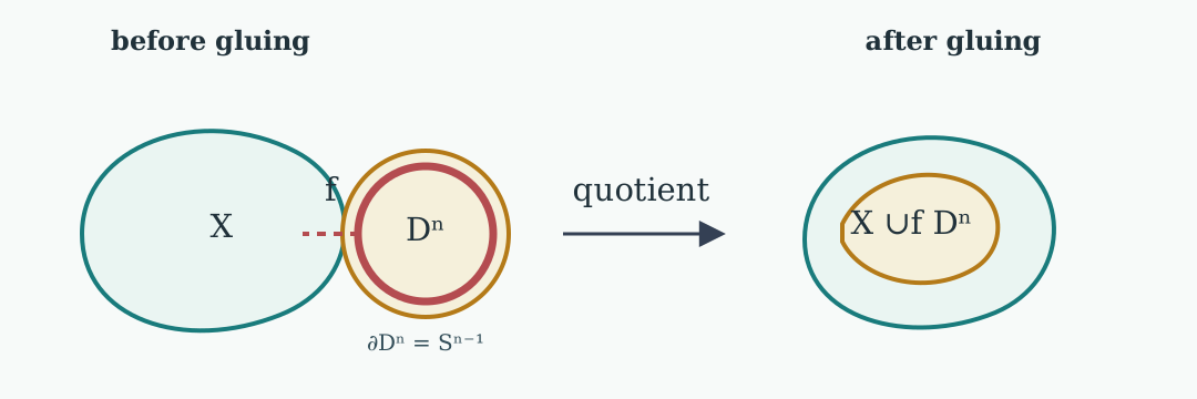
How to read it. The disk is still separate on the left. Only its boundary is identified with $X$; the disk interior becomes the new open cell on the right.
Characteristic map. For an attached cell $e^n$, the quotient map $D^n\to X\cup_fD^n$ is a characteristic map. Its restriction to the interior of $D^n$ is a homeomorphism onto $e^n$, while its restriction to $S^{n-1}$ is the attaching map followed by the inclusion of $X$ into the quotient.
Two immediate examples fix the conventions. Attaching $D^n$ to a point by the constant map gives $S^n$, because every boundary point is collapsed to the same point. Attaching one $n$-disk to another along the identity map on their common boundary gives
$$ D^n\cup_{\operatorname{id}_{S^{n-1}}}D^n\cong S^n; $$the two disks become the two hemispheres. The same symbol $D^n$ can therefore produce different spaces; the attaching map is part of the data.
3. CW complexes
Term bridge. The letters CW refer to two conditions. Closure-finite means that the closure of each cell is contained in the union of finitely many cells. Weak topology means that openness in the whole union is tested on every skeleton. The $n$-skeleton $X^n$ is the part made from cells of dimension at most $n$.
A CW complex is built one skeleton at a time. Start with a discrete set $X^0$ of $0$-cells. Having constructed the $(n-1)$-skeleton $X^{n-1}$, choose attaching maps
$$ \varphi_\alpha:S^{n-1}\longrightarrow X^{n-1} $$and form
$$ X^n=X^{n-1}\cup_{\{\varphi_\alpha\}}\coprod_\alpha D^n_\alpha. $$The index $\alpha$ allows several $n$-cells. The union $X=\bigcup_{n\geq0}X^n$ is given the weak topology: a set $U\subseteq X$ is open if and only if $U\cap X^n$ is open in $X^n$ for every $n$. A finite-dimensional complex stops at some $X^n$; an infinite-dimensional one does not.
The $n$-skeleton $X^n$ contains all cells of dimension at most $n$. An open cell is the image of the interior of one disk. The characteristic map need not be injective on the boundary, but it is a homeomorphism from the disk interior onto the open cell.
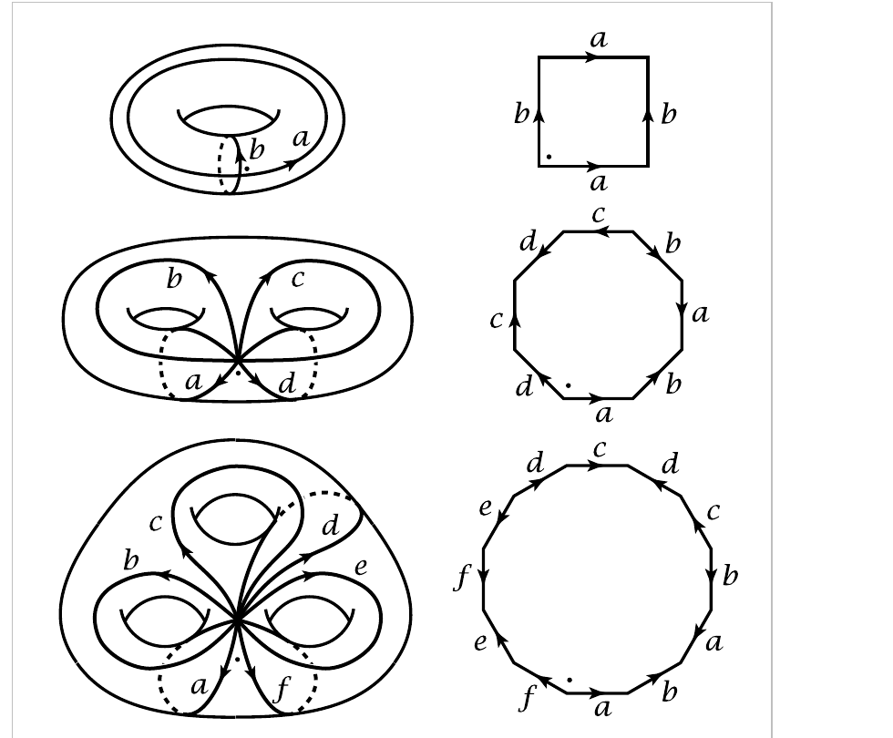
How to read it. Each polygon on the right is a boundary word; the surface on the left is the quotient obtained by making the indicated edge identifications.
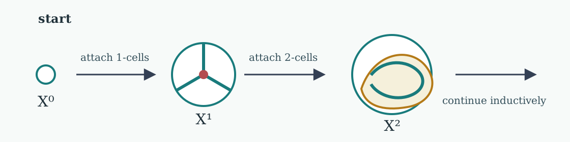
How to read it. The arrows are operations: first attach edges to make $X^1$, then attach disks to make $X^2$, and continue in the same way.
Three standard cell structures. A graph is a $1$-dimensional CW complex: vertices are $0$-cells and edges are $1$-cells. The sphere $S^n$ has one $0$-cell and one $n$-cell, attached by a constant map. Real projective space has one cell in each dimension $0,1,\ldots,n$; the attaching map of the $k$-cell is the quotient map $S^{k-1}\to\mathbb{RP}^{k-1}$ identifying antipodal points. These descriptions are not merely labels: they specify the maps needed to reconstruct the spaces.
The torus has a particularly efficient structure: one $0$-cell, two $1$-cells, and one $2$-cell. Its $1$-skeleton is a wedge $S^1\vee S^1$, and the boundary of the $2$-cell travels once around the first circle, once around the second, once backwards around the first, and once backwards around the second. In the fundamental group this boundary word becomes the commutator. The cell picture already predicts where the relation in $\pi_1(T^2)$ comes from; the calculation will appear after the fundamental group is defined.
4. Quotients and other operations
If $(X,A)$ is a CW pair, then $X/A$ inherits a CW structure. The cells outside $A$ remain, and the whole subcomplex $A$ becomes one new $0$-cell. In particular,
$$ D^n/S^{n-1}\cong S^n. $$If $(X,x_0)$ and $(Y,y_0)$ are based spaces, their wedge sum is
$$ X\vee Y=(X\amalg Y)/(x_0\sim y_0). $$Term bridge. A based space is a space with a chosen point. The wedge sum uses those points as its single gluing point. This choice is essential when later defining based loops and fundamental groups.
The wedge point is part of the construction; without chosen basepoints the notation has no defined meaning. In the standard CW structure on a torus, for instance, the $1$-skeleton is $S^1\vee S^1$ because the two circle cells meet at the single $0$-cell.
The suspension of $X$ is the quotient $\Sigma X=(X\times I)/\sim$, where all points of $X\times\{0\}$ are equivalent, all points of $X\times\{1\}$ are equivalent, and there are no other identifications.
It is the union of two cones on $X$. Since $\Sigma S^n\cong S^{n+1}$, suspension raises the dimension of the sphere by one. A map $f:X\to Y$ induces $\Sigma f:\Sigma X\to\Sigma Y$ by applying $f$ to the $X$-coordinate; this is why suspension is an operation on maps as well as on spaces.
Term bridge. The cone $CX$ collapses one end of $X\times I$ to a point. The suspension uses two cones and keeps their bases identified along $X$. It is therefore a quotient construction with two distinguished suspension points.
5. Two ways to recognize a homotopy equivalence
The first criterion concerns collapsing a subspace. If $(X,A)$ is a CW pair and $A$ is contractible, then the quotient map
$$ X\longrightarrow X/A $$is a homotopy equivalence. The CW hypothesis controls the gluing; contractibility of $A$ supplies the homotopy that replaces all of $A$ by one point. This is a theorem to be proved later in Hatcher, not a rule that may be applied to arbitrary subspaces without hypotheses.
Term bridge. A space is contractible if its identity map is homotopic to a constant map. It has the homotopy type of one point, but the theorem above still needs the CW-pair hypothesis to justify collapsing it inside $X$.
For a finite graph, the criterion has a direct form. If an edge has two distinct endpoints, collapse that edge to a point. The quotient graph has one fewer edge and is homotopy equivalent to the original graph. Repeating this removes every non-loop edge. What remains is a wedge of circles, one for each independent cycle.
The second criterion concerns attaching maps. If $(Y,A)$ is a CW pair and $f,g:A\to X$ are homotopic, then
$$ X\cup_fY\simeq X\cup_gY. $$The homotopy must be defined on the attaching subspace $A$; changing the map only at a few boundary points is not enough. This criterion is the precise version of the geometric statement that one may slide a piece of a cell attachment continuously without changing the homotopy type.
6. A complete attaching-map calculation
Let $X=S^1$ and let $f_n:S^1\to S^1$ have degree $n$. Attach a disk along $f_n$:
$$ M_n=S^1\cup_{f_n}D^2. $$The integer $n$ records how many times the boundary of the disk winds around the original circle, with sign recording orientation. The resulting space is a CW complex with one cell in each of dimensions $0$, $1$, and $2$.
Term bridge. For a map $f:S^1\to S^1$, its degree is the signed winding number: how many times the source circle covers the target circle, counting orientation. Degree $0$ is null-homotopic; degree $1$ is the identity up to homotopy.
Three values show why the attaching map matters. For $n=0$, the boundary is attached to one point, so
$$ M_0\cong S^1\vee S^2. $$For $n=1$, the disk is attached along the identity map of the circle, so $M_1\cong D^2$ and is contractible. For $n=2$, the space is the standard cell model of $\mathbb{RP}^2$: the $1$-skeleton is $\mathbb{RP}^1\cong S^1$, and the $2$-cell wraps its boundary twice.
The cellular chain complex makes the distinction numerical. With one generator in dimensions $2$ and $1$, the boundary map $C_2\to C_1$ is multiplication by $n$; hence
$$ H_1(M_n;\mathbb Z)\cong\mathbb Z/n\mathbb Z, $$where $\mathbb Z/0\mathbb Z$ means $\mathbb Z$. This is the first example in which a geometric winding number becomes an algebraic boundary map. The full justification belongs to the cellular homology chapter, but the attaching construction already identifies the integer that homology will detect.
Reading rule. Whenever a source says that a space is “obtained by attaching a cell,” record four items: the old space $X$, the disk dimension $n$, the attaching sphere $S^{n-1}$, and the map $f:S^{n-1}\to X$. Without the fourth item the construction is incomplete.
7. Exercises for this reading
- Prove directly that $[0,1]/(0\sim1)$ is homeomorphic to $S^1$ using the quotient property.
- Describe $\mathbb{RP}^2$ as a $0$-cell, a $1$-cell, and a $2$-cell. Identify the degree of the attaching map of the $2$-cell.
- Collapse a chosen non-loop edge in a finite connected graph and describe the induced change in the number of vertices, edges, and independent cycles.
- For $M_n=S^1\cup_{f_n}D^2$, explain geometrically why the boundary map in the cellular chain complex is multiplication by $n$.
The next note will read Hatcher Chapter 1 through the fundamental group of the circle, van Kampen’s theorem, and the first use of a cell structure in a homotopy calculation.
Sources
- Allen Hatcher, Algebraic Topology, Chapter 0, pp. 5–13 (PDF pp. 14–22): author’s PDF.
- Andrew Lin, notes for Zhenkun Li’s Stanford MATH 215A, pp. 1–5: course notes.
- The previous note in this series: Homotopy and deformation retractions.