We begin this analysis supplement with Sheldon Axler, Measure, Integration & Real Analysis, Sections 1B, 2B–2D, 3A–3B, and 7A–7B. The definitions below use real-valued functions; Cheng Wei’s Real Variable Theory, Chapters 3–5, provides a Chinese comparison. Our aim is to understand why integration leads to spaces in which functions are identified when they agree almost everywhere. These spaces will be used in the next note on weak derivatives, and later in analytic approaches to Hodge theory.
In Axler’s Example 1.14, the function $f=\mathbf 1_{\mathbb Q\cap[0,1]}$ equals $1$ at rational points of $[0,1]$ and $0$ elsewhere. Here $\mathbb Q$ denotes the rational numbers and $\mathbf 1_E$ denotes the indicator of a set $E$. Every interval of positive length contains rational and irrational points, so every lower Riemann sum is $0$ and every upper Riemann sum is $1$. The Riemann integral therefore does not exist. Lebesgue integration will give this function integral $0$, because its nonzero set has measure $0$.
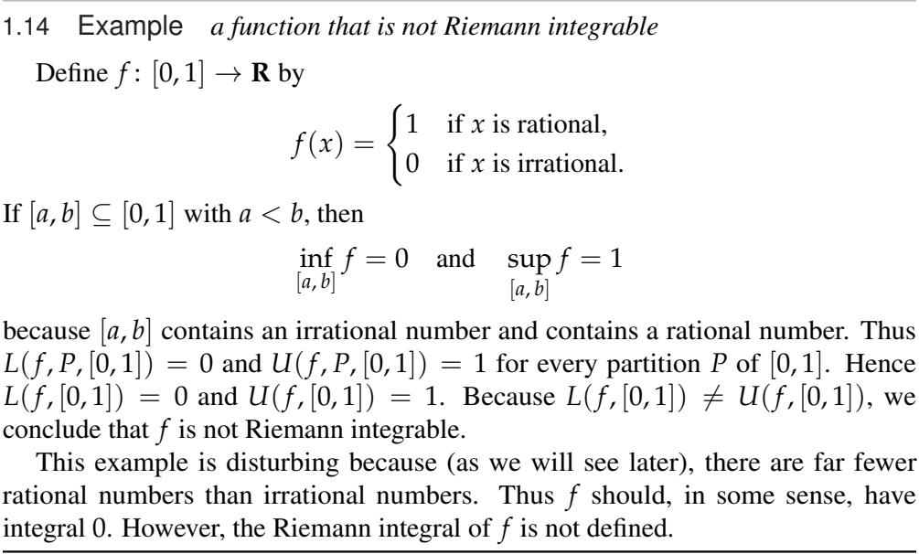
Sheldon Axler, Measure, Integration & Real Analysis, Example 1.14, printed p. 9 (PDF p. 24). Cropped from the author's PDF; CC BY-NC 4.0. The original uses lower and upper sums to make the failure precise.
1. A measure is a rule for size
A measurable space is a pair $(X,\mathcal M)$. Here $X$ is a set and $\mathcal M$ is a collection of subsets of $X$ called the measurable sets. The collection $\mathcal M$ must satisfy
$$ \varnothing\in\mathcal M,\qquad E\in\mathcal M\Longrightarrow X\setminus E\in\mathcal M, $$and
$$ E_1,E_2,\ldots\in\mathcal M \Longrightarrow \bigcup_{j=1}^{\infty}E_j\in\mathcal M. $$Such a collection is called a sigma-algebra. Here $E_j$ is the $j$th set in a sequence and $X\setminus E$ is its complement in $X$. Closure under countable intersections follows by taking complements. The symbol $\mathcal M$ records which subsets may be measured; the measure itself assigns their sizes. If $X$ is a topological space, its Borel sigma-algebra is the smallest sigma-algebra containing all open sets. On $\mathbb R$ this includes open and closed intervals.
A measure on $(X,\mathcal M)$ is a function
$$ \mu:\mathcal M\longrightarrow[0,\infty] $$such that $\mu(\varnothing)=0$ and, whenever the measurable sets $E_j$ are pairwise disjoint,
$$ \mu\left(\bigcup_{j=1}^{\infty}E_j\right) =\sum_{j=1}^{\infty}\mu(E_j). $$The triple $(X,\mathcal M,\mu)$ is a measure space. The value $\infty$ is allowed. For Lebesgue measure $\lambda$ on $\mathbb R$,
$$ \lambda([a,b])=b-a\qquad(a\leq b). $$Taking $a=b$ gives $\lambda(\{a\})=0$. If $E=\{x_1,x_2,\ldots\}$ is countable with distinct points, countable additivity gives $\lambda(E)=\sum_j\lambda(\{x_j\})=0$. In particular, $\lambda(\mathbb Q\cap[0,1])=0$. A null set is a measurable set of measure $0$. The Lebesgue sigma-algebra contains the Borel sets and every subset of a Borel null set; we use this complete sigma-algebra when discussing Lebesgue measure.
2. Measurable functions and indicator functions
Let $(X,\mathcal M)$ be a measurable space. A function
$$ f:X\longrightarrow[-\infty,\infty] $$is measurable if, for every real number $a$,
$$ \{x\in X:f(x)>a\}\in\mathcal M. $$The set inside braces consists of points where $f$ exceeds the threshold $a$. Requiring every such set to be measurable lets us measure how often the function takes values in a given range. Equivalently, the preimage $f^{-1}(B)=\{x:f(x)\in B\}$ of every Borel set $B$ in the extended real line is measurable. Every continuous real-valued function is Borel measurable; a measurable function need not be continuous.
For a measurable set $E$, its indicator function is
$$ \mathbf 1_E(x)= \begin{cases} 1,&x\in E,\\ 0,&x\notin E. \end{cases} $$Indicator functions are the basic building blocks for integration. They translate a set into a function.
3. The Lebesgue integral
A nonnegative simple function has the form
$$ s=\sum_{k=1}^m a_k\mathbf 1_{E_k}, \qquad a_k\geq0, $$Here $m$ is a positive integer, the coefficients $a_k$ are finite real numbers, and the sets $E_k$ are measurable and pairwise disjoint. Thus $s$ takes only finitely many values. Define its integral by
$$ \int_Xs\;d\mu=\sum_{k=1}^m a_k\mu(E_k). $$The notation $d\mu$ specifies the measure used for integration, and we use the convention $0\cdot\infty=0$. Refining two representations into disjoint measurable pieces shows that the value of the integral does not depend on how $s$ is represented.
For a nonnegative measurable function $f$, define
$$ \int_Xf\;d\mu =\sup\left\{\int_Xs\;d\mu: s\text{ is simple and }0\leq s\leq f\right\}. $$The supremum is the least upper bound of all these simple-function integrals, and it may be infinite. This is the simple-function formulation in Axler’s result 3.9, equivalent to his definition by lower Lebesgue sums. For a real-valued measurable function, set
$$ f^+=\max\{f,0\},\qquad f^-=\max\{-f,0\},\qquad f=f^+-f^-. $$If
$$ \int_Xf^+\;d\mu+\int_Xf^-\;d\mu<\infty, $$then $f$ is integrable and
$$ \int_Xf\;d\mu =\int_Xf^+\;d\mu-\int_Xf^-\;d\mu. $$The functions $f^+$ and $f^-$ are its positive and negative parts; their sum is $|f|$. Thus integrability means $\int_X|f|\;d\mu<\infty$. On Euclidean domains we write $dx$ for Lebesgue measure instead of $d\lambda$. The Lebesgue integral agrees with the Riemann integral whenever the latter exists.
Returning to the opening example. By the definition for simple functions, $\int_{[0,1]}\mathbf 1_{\mathbb Q\cap[0,1]}\;d\lambda=\lambda(\mathbb Q\cap[0,1])=0$. Its everywhere-discontinuous representative and the identically zero function have the same integral. This does not make them the same pointwise function; it means integration cannot distinguish their values on a null set.
4. Convergence theorems
The main advantage of the Lebesgue integral is that it has precise rules for passing to limits.
Suppose $f_n$ are nonnegative measurable functions with $0\leq f_1\leq f_2\leq\cdots$ and $f_n(x)\to f(x)$. The monotone convergence theorem says
$$ \int_Xf\;d\mu=\lim_{n\to\infty}\int_Xf_n\;d\mu. $$The value on either side may be infinite. For signed functions, the dominated convergence theorem says that if measurable real-valued functions $f_n$ converge to a measurable $f$ almost everywhere, and one nonnegative integrable function $g$ satisfies
$$ |f_n|\leq g\quad\text{almost everywhere, for every }n, $$then
$$ \lim_{n\to\infty}\int_Xf_n\;d\mu =\int_Xf\;d\mu. $$The limit $f$ is integrable as well. Here almost everywhere, abbreviated a.e., means outside a measurable null set. The hypotheses of these theorems are essential. On $(0,1)$, let $f_n=n\mathbf 1_{(0,1/n)}$. Every fixed $x>0$ eventually lies outside $(0,1/n)$, so $f_n(x)\to0$, but $\int_0^1 f_n\;dx=1$ for every $n$. Pointwise convergence alone does not permit interchange of limit and integral: mass can concentrate near a point.
5. The spaces $L^p$
For $1\leq p<\infty$, first collect the measurable real-valued functions with finite $p$th-power integral:
$$ \mathcal L^p(X,\mu) =\left\{f:X\to\mathbb R\text{ measurable}: \int_X|f|^p\;d\mu<\infty\right\}. $$The associated norm is
$$ \lVert f\rVert_p =\left(\int_X|f|^p\;d\mu\right)^{1/p}. $$On actual functions this is only a seminorm: it can vanish for a function that is not pointwise zero. Define $f\sim g$ when $f=g$ a.e., and let $[f]$ denote the equivalence class of $f$. The space $L^p(X,\mu)$ is the quotient $\mathcal L^p(X,\mu)/\!\sim$, with $\lVert[f]\rVert_p=\lVert f\rVert_p$. Now norm zero means the zero equivalence class. It is customary to write $f\in L^p$ and leave the equivalence class implicit. Evaluation at a single point is generally not well defined on these classes.
The space $L^\infty(X,\mu)$ consists of measurable functions that are essentially bounded. Its norm is
$$ \lVert f\rVert_\infty =\operatorname*{ess\;sup}_{x\in X}|f(x)|, $$Explicitly, the essential supremum is $\inf\{M\geq0:|f|\leq M\text{ a.e.}\}$. It measures the smallest bound that holds outside a null set. As before, $L^\infty$ identifies representatives that agree a.e.
If $1<p<\infty$ and $q$ satisfies
$$ \frac1p+\frac1q=1, $$then Holder’s inequality is
$$ \int_X|fg|\;d\mu \leq\lVert f\rVert_p\lVert g\rVert_q. $$Here $f\in L^p$, $g\in L^q$, and $q=p/(p-1)$ is the conjugate exponent of $p$. The endpoint pair $p=1$, $q=\infty$ is also valid. For $p=q=2$, this is the integral form of Cauchy–Schwarz. It will ensure that the products in the weak-derivative identities are integrable.
The Minkowski inequality says
$$ \lVert f+g\rVert_p\leq\lVert f\rVert_p+\lVert g\rVert_p. $$Minkowski gives the triangle inequality for the norm. The completeness theorem, Axler’s result 7.24, says that every Cauchy sequence in this norm has a limit in $L^p$. Thus $L^p$ is a Banach space. For $p=2$, the real inner product $\langle f,g\rangle=\int_Xfg\;d\mu$ makes it a Hilbert space, a complete inner product space.
A complete integrability calculation. Let $\alpha\geq0$ and $f(x)=x^{-\alpha}$ on $(0,1)$. Put $\beta=\alpha p$ and choose a cutoff $0<\varepsilon<1$. For $\beta<1$, integrating first over $(\varepsilon,1)$ gives $\int_\varepsilon^1x^{-\beta}\;dx=(1-\varepsilon^{1-\beta})/(1-\beta)$. Letting $\varepsilon\downarrow0$ gives $\int_0^1x^{-\beta}\;dx=1/(1-\beta)$. For $\beta=1$ the integral is $-\log\varepsilon$, and for $\beta>1$ the power term diverges. Hence $f\in L^p(0,1)$ exactly when $\alpha p<1$, with $\lVert f\rVert_p=(1-\alpha p)^{-1/p}$. In particular, $x^{-1/2}$ belongs to $L^1(0,1)$ but not $L^2(0,1)$.
6. Why this supplement belongs here
Our main observation is that $L^p$ changes the notion of equality before introducing a notion of distance. Null-set values are discarded; the norm then controls the remaining function in an integral sense. This explains why pointwise differentiation will be unsuitable in the next note: it must be replaced by a definition that depends only on the a.e. class.
Basic homotopy and singular homology require none of this analysis. Smooth differential forms and classical de Rham cohomology can also be developed before Sobolev theory. These supplements prepare the later analytic step, where forms have $L^2$ coefficients and elliptic estimates enter Hodge theory.
In Supplement II, integration by parts will provide that definition and lead to Sobolev spaces.
7. Exercises for this reading
- Prove that every countable subset of $\mathbb R$ has Lebesgue measure $0$.
- Compute $\int_0^1x^{-\alpha}\;dx$ and determine exactly when it is finite.
- Suppose $f$ and $g$ are measurable and agree almost everywhere. Show that if $f\in\mathcal L^p$, then $g\in\mathcal L^p$ and $\lVert f\rVert_p=\lVert g\rVert_p$.
- For $p=2$, explain why $\langle f,g\rangle=\int_Xf\;g\;d\mu$ is an inner product after identifying functions that agree almost everywhere.
Sources
- Sheldon Axler, Measure, Integration & Real Analysis, 12 June 2026 PDF: Sections 1B (pp. 9–11), 2B–2D (pp. 25–59), 3A–3B (pp. 74–98), and 7A–7B (pp. 194–208). Author’s page; author’s PDF; archived PDF; CC BY-NC 4.0. Printed page $r$ is PDF page $r+15$ in this edition.
- John K. Hunter, Measure Theory: course page and lecture notes.
- Cheng Wei, Real Variable Theory (Chinese), Chapters 3–5, pp. 41–92: author’s page and lecture notes.